GOLD FORECAST REPORT OPTION OF SIRIUS

A forecast of gold prices was developed in 2006 and is available as the “Gold Forecast” report option of the Sirius astrology program. This gold forecast is based on minor aspects, also sometimes referred to as harmonic aspects or harmonics. It produces a strong correlation of predicted gold prices and actual gold prices (see http://astrosoftware.com/goldforecast.htm).

The statistical analysis performed however may have given biased or inaccurate results for two reasons:

These two issues are addressed in a reanalysis of the gold forecast, and the new analysis confirms the previous findings. This confirmation of the earlier analysis may represent one of the strongest validations of a measurable effect of astrological variables, especially given the recent reanalysis of Gauquelin studies which suggest that there are limitations and problems in the Gauquelin research that were previously unidentified. Click on the links below to view the articles.

The Gold Forecast report option of Sirius predicts relatively short-term forecasts of gold prices. Gold prices from January 1, 1975 to June 30, 2006 were analyzed. The forecast produces relatively short-term forecasts based on the angular relationship of the geocentric positions of the planets measured along the ecliptic plane.

The forecast based on Sun and Jupiter in 7th harmonic produces an expected rise in gold prices approximately every seven weeks with one exception: when the Sun is 6/7 of the circle past Jupiter and the conjunction is “jumped over” and the next peak is predicted to occur when the Sun is 1/7 past Jupiter and thus there are approximately 14 weeks between the occurrence of the 6/7 and 1/7 aspect.

There are six predicted rises in gold prices (the 1/7, 2/7, 3/7, 4/7, 5/7, and 6/7 aspects of Sun and Jupiter) which occur over a period of about 13 months. An orb of slightly less than two degrees is allowed and each rise in gold prices is therefore forecasted to last about four days. All durations vary because the speeds of planets vary over time.

The forecast based on 7th harmonic aspects of Sun and Jupiter is simple and elegant. The predicted gold price is predicted to begin rising as Sun and Jupiter are within two degrees of one of these six aspects, the gold price reaches its peak when the aspect is exact, and the price declines as the planets separate from each other by about a 2 degree orb again. The predicted rise and fall of gold prices over these time periods of approximately four days is expected to conform to a gradual increase similar to a sine wave. There are no autoregressive effects or other effects based on a cyclic analysis or the effect of earlier prices on later prices. There are also no time delays in the effect of the astrological variable.

In the terminology used by research methodologists, the astrological influence is an extraneous time-varying covariate. The astrological variable is clearly extraneous because planetary orbits are determined by mathematical formulae that are independent of human behavior.

Another elegant feature of this forecast is that all 7th harmonic aspects are given equal weight. The 1/7 aspect, for example, is expected to increase gold prices by the same amount as a 2/7 aspect and 3/7 aspect would. All of the harmonic aspects are also given the same orb. The theoretical framework for this study is harmonic astrology as described by John Addey and specific interpretations elaborated by David Cochrane. In harmonic astrology, angles between planets that are within orb of a fraction have a similar, but not identical, effect if that aspect expressed as a fraction has the same denominator. This expectation is based on the concept that astrological aspects operate through a kind of wave function that has as yet been undetected by any instruments.

Gold prices are posted on daily trading days, which are weekdays except major holidays. There are consequently about 255 trading days each year. A forecasted price can be produced for every day of the year but gold prices are given only on trading days. This issue can be viewed as a missing data problem in that gold prices would be available every day if the services were provided to give gold prices as people will buy and sell gold every day and virtually all of the forces that affect gold prices are in effect on weekends as well. As a crude analogy, one might say that a person still has a pulse even if the pulse is not measured. The “missing” gold prices can be ignored or imputed. We can get a sense of the effects of missing gold prices by looking at a graph of actual and predicted gold prices over a 3-month period with the missing gold prices imputed, as shown in Figure 1.

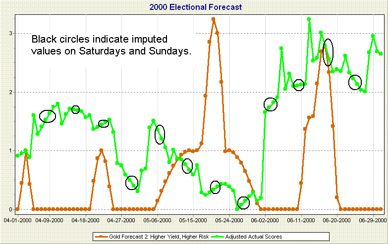
Figure 1. 3-Month Forecast with Imputed Values on Weekends Identified

As shown in Figure 1, the imputed values for days on non-trading days, are values that are determined by a simple linear interpolation between the prices on the preceding Friday and following Monday. Over the 3-month period the linear interpolation used to impute values for weekends appears to be reasonable. Given that the price of gold must change from its price on Friday to its price on Monday, the assumption of a steady linear change over Saturday and Sunday is reasonable and represents the likely mean values if prices varied randomly from the price on Friday to the price on Monday. As can be seen by looking at the graph in Figure 1, the amount of deviation that is likely from these imputed prices is not likely to drastically change the overall relationship of the predicted prices (red line) to the actual prices (green line). For this analysis we used imputed values of the gold prices on non-trading days, a shown in Figure 1.

Note that the predicted prices shown in Figure 1 are based on more astrological factors than the Sun-Jupiter 7th harmonic aspects. A Sun-Jupiter 7th harmonic aspect is likely to occur only one time on average over the three month period so there would be only one predicted period of about 4 days when prices would increase if only Sun-Jupiter aspects were used to predict a rise in gold prices.

There are two gold forecasts produced by the Gold Forecast report option of Sirius. One of these forecasts is called the “Higher Yield, Higher Risk” forecast because the mean correlation based on this formula is higher than the other forecast but the range of correlations is also greater. The difference between the mean, minimum, and maximum correlations between the two forecasts is not great. In the present study only the Higher Yield, Higher Risk forecast is analyzed.

In retrospect, the Lower Yield, Lower Risk forecast is arguably a better candidate for research because the collection of astrological variables are more consistent, i.e., they are simpler and more elegant than the variables used in the Higher Yield, Higher Risk forecast. Both forecasts have 36 items, and 7 of the 36 items are harmonic aspects, while the other 29 items are asymmetric isotraps (explained below). The 7 harmonic aspects in the Lower Yield, Lower Risk formula are between Sun and Jupiter or Jupiter and Neptune and are 7-based harmonics or conjunctions. The 7-based aspects are harmonics 14, 21, 28, and 35 between Sun and Jupiter. The Higher Yield, Higher Risk formula also includes 5th harmonic aspects between Venus and Mars and between Mars and Jupiter, a trine aspect between Sun and Saturn and therefore uses more planets in more harmonics than the Lower Yield, Lower Risk formula.

In the future a replication of the current study with the Lower Yield, Lower Risk formula is planned and similar results are expected because the differences in mean, minimum, and maximum correlations using the two formulae are small, and the lower risk of the Lower Yield, Lower Risk formula compensates to some extent for the lower correlations because the correlations are more consistently positive and thus there is likely less variability in the correlations.

In addition to harmonic aspects, both formulae use midpoint-to-midpoint aspects as predictors. More specifically, 18th harmonic midpoint-to-midpoint aspects between Sun, Mars, Jupiter, and Uranus and 3rd and 6th harmonic midpoint-to-midpoint aspects between Mars, Jupiter, Uranus, and Neptune are used as predictors. Midpoint-to-midpoint relationships are regarded as highly important in the theoretical framework of symmetrical astrology. Cochrane has written extensively about their importance in compatibility and in relationship to arabic parts. See, for example, http://www.astrosoftware.com/Symmetries.htm and http://www.astrosoftware.com/ArabicParts.htm).

STATISTICAL ANALYSIS: Meta-analysis of 3-month Periods

As discussed above, the model for the gold forecast is elegant and simple. The only variables are extraneous time-varying covariates that affect the dependent variable (gold prices) without any time delay. There are not any autoregressive or cyclic effects that are considered in this study. There is, however, one issue in the statistical analysis that presents an obstacle: how to measure the effect of a time-varying covariate that is expected to have an effect for a relatively short period of time over time series data that extends for a relatively long period of time. In this case there are 31 ½ years of gold data and each of the time-varying covariates (the astrological variables) is expected to affect gold prices over a period of a few days to a few weeks. If gold prices were relatively stable over the 31 years, the long-term effects would not overwhelm short-term trends but gold prices, like many financial measures and indicators, have very dramatic long-term trends. Gold prices may, for example, go up or down in a striking manner over a period of months or years. These larger trends overwhelm the short term effects in a correlation that spans the entire 31 years. The graph in Figure 2 demonstrates the problem.

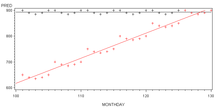
Figure 2: Example of Short-Term Forecast Overwhelmed by Long-Term Trend

The red “+” characters in Figure 2 represent the actual data. The linear fit to this data is shown by the red line. The black “+” characters near the top of the graph represent the predicted values based on an extraneous time-varying covariate that is able to only forecast behavior in relationship to the random expected behavior over a short period of time. A horizontal regression line is drawn through these forecasted values. Notice that the forecasted values are perfect. The actual values are grouped in a series of five values that starts high goes gradually down to the third value of the five and then back up. If we divide the data into 6 separate analyses of 5 values each, then the r correlation coefficient will be a perfect 1.0. However, the r correlation coefficient for the data in this graph is only .07 and the p value is .71 indicating that our predicted values have no relationship to the actual values. The horizontal black regression line for predicted values and the ascending red regression line of actual values reinforces this point. The predicted values do not do a very good job of correlating with actual values even though over a 5-day period the correlation is perfect.

For the interest of anyone who may wish to “play” with this issue, the SAS code to generate the above graph is given in Table 1.

Table 1. SAS Code that generates the data in Figure 2.

options ps=60 ls=78;
Data One;
INPUT MONTHDAY 1-4 ACTUAL 6-8 PRED 10-12;
DATALINES;
0101 650 900
0102 640 890
0103 635 885
0104 640 890
0105 650 900
0106 700 900
0107 690 890
0108 685 885
0109 690 890
0110 700 900
0111 750 900
0112 740 890
0113 735 885
0114 740 890
0115 750 900
0116 800 900
0117 790 890
0118 785 885
0119 790 890
0120 800 900
0121 850 900
0122 840 890
0123 835 885
0124 840 890
0125 850 900
0126 900 900
0127 890 890
0128 885 885
0129 890 890
0130 900 900
* PROC PRINT;
SYMBOL1 V=plus C=black I=R;
SYMBOL2 V=plus C=red I=R;
PROC GPLOT DATA=ONE; PLOT (PRED ACTUAL) * MONTHDAY /OVERLAY;
PROC CORR DATA=ONE SSCP CSSCP COV;
RUN;
QUIT;

To summarize, the detection of short-term effects of extraneous time-varying covariates over time series data over a relatively long period of time is overwhelmed by strong long-term trends in the data. The strong long-term trend in the data in Figure 2 is the positive trend upwards over time. Although the data in Figure 2 is idealized in order to illustrate the point, the same principles are in effect in the analysis of the astrological variables used in the gold forecast.

Three possible ways to address this issue come to mind:
(1) Find astrological variables that predict long-term trends so that the complete forecast is possible. This option is theoretically unattractive to me because I doubt that astrological variables have a clear association with long term trends as these trends are most likely affected by a complex interaction of a great many variables, including social policies in various countries, overall economic trends, etc.
(2) A kind of correction for long-term effects may be possible. For example, in the idealized data in Figure 2, the data could be corrected for the linear effect. However, with complex real-world data, establishing a sound procedure for a correction factor would be extremely complex.
(3) Divide the data into smaller sections of time and obtain a set of correlation values. This approach is intuitively appealing because the theory proposed is that short-term trends can be predicted so dividing the data into groups of short-term trends reflects clearly and directly the hypothesis being proposed.

One might expect that the best statistical procedures for analyzing this data would be clearly presented in books and research papers. However, after a thorough search through a great many online sources of books on time line series and longitudinal data analysis, and a search for relevant papers in research journals, I was unable to find one that addressed this issue. Not having expertise in this particular area of research methodology, I may have easily overlooked this information. The difficulty in locating this information may be surprising in that the issue seems simple, basic, and straightforward while much more complex issues are addressed in time series analysis, but it is perhaps not surprising in that research methods are typically developed out of real-world needs. Much of the progress in time series analysis and longitudinal data analysis evolves from issues encountered in medical, economic, and educational studies. Encountering an analogous situation where an extraneous time-varying covariate has short-term effects that are overwhelmed by long-term trends in time series data appears to be unlikely. Research on measurable effects of astrological variables is not only outside the mainstream of academia and research institutes but largely outside the mainstream of astrology as well, which is more focused on issues of personality, qualitative effects, divination, and psychic or metaphysical perception rather than measurable effects.

When the gold forecast option of Sirius was developed in late 2006, the decision was made to divide the 31 ½ years of data into 126 3-month periods and thus produce 126 Pearson r correlation values and then analyze the total effect of these 126 correlations with a kind of meta-analysis. Even though meta-analysis is typically associated with obtaining a synthesized result from separate studies, the assumptions of the meta-analysis statistical methods are appropriate for analyzing the 126 correlations produced by the gold forecast. In fact, the consistency of the data in terms of the manner in which it is gathered and the similar n (number of data) in each 3-month period is very consistent with the assumptions of meta-analysis statistical methods and is less likely to violate the assumptions of the statistical analysis than a meta-analysis of separate studies.

REANALYSIS USING DIFFERENT STARTING DATES

Having been unsuccessful in identifying a precedent for measuring short-term effects of time-varying covariates on time series data with strong long-term trends, the statistical procedure that I used in 2006 appears to be reasonable. There are two limitations in the analysis of the data that was performed in 2006 that are addressed in the current reanalysis of the data:

(1) In the analysis of the data performed in 2006 the starting dates of each 3-month period were January 1, April 1, July 1, and October 1. These are the dates that were used in the study of the data to develop the two AstroSignatures (the Low Yield, Low Risk and High Yield, High Risk sets of astrological variables). An analysis needs to be conducted using other starting points to see if the results are sufficiently robust to be present when different starting dates. The gold forecast is the result of exploratory research rather than a hypothesis test and the significance level of the results do not “prove” anything. Rather, they are used to help guide a path of exploration that may eventually lead to a definitive finding. Analyzing the results using different starting dates is a first step in determining if the findings are generalizable even at a most basic level. If the statistical significance is greatly impacted by changing the starting dates, then the exploratory research has been found to be ineffective from the outset.

(2) The meta-analysis was performed using a rarely used software program developed by a professor at the University of Miami primarily for pedagogical purposes. The rapid expansion of the R statistical language system in recent years makes it an attractive tool. In this reanalysis of the High Yield, High Risk AstroSignature developed in 2006, the meta-analysis was performed using R.

In the reanalysis of the gold data, 126 correlations between the predicted and actual gold prices were produced using the Sirius 1.2 software. In Sirius 1.2 a new feature has been added to allow automatic saving to file of all 126 analyses with results saved to file in a CSV file that can be used by R code, other statistical software, and spreadsheet software. The analysis was repeated with different starting dates separated by 10 to 15 days. In Table 2 the starting dates in the first quarter of each year, the p value and mean r correlation value are given. The other starting dates are on the same day of the month every 4 months so that, for example, for the data beginning on February 26, correlations are for 3-month periods beginning February 26, May 26, August 26, and November 26.

Table 2. Probabilities and Mean Correlation (r) of Predicted and Actual Gold Prices for Eight Different Starting Dates of the Gold Forecast

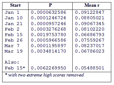At the bottom of Table 2 is an additional set of values for the 3-month period beginning February 15, but with the highest two correlations removed. The reason for performing this analysis is evident by inspecting the graphs in Figure 3. The second graph in Table 3 shows the 126 correlation values and standard errors. Two of the 126 correlations were much higher than the other 124, as can be seen in the discontinuous jump from the previous values in the bottom two r correlation values shown in this graph. In the third graph is the same data plotted with these two very high correlations removed. Note that these correlations are not outliers and should not be removed! They were removed only for the purpose of seeing how much affect they had on the mean correlation and p value for the analysis beginning on February 15. Note also that mean correlations are slightly different from a mean value that would be calculated by simply adding the 126 correlations and dividing by 26. These are mean values based on the meta-analysis and take into account the number of dates in each 3 month period, which varied only slightly between 90 and 92.

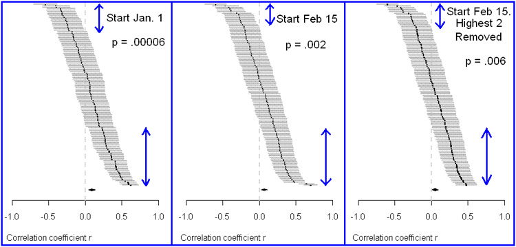
Figure 3. Graph of 126 correlations of 3-month periods between predicted and expected gold prices.
The gray lines extending from the correlation values indicates the standard error of measurement.
The third graph has the highest two correlations removed so is based on 124 correlations instead of 126.

The mean r values shown in Table 2 range from .067 to .091. As expected, the highest correlation occurs on the dates on which the AstroSignature was developed, January 1. The correlations did degrade on other dates. Interestingly, the correlations do not gradually become worse as the starting date is increased from January 1, although the date farthest from the Jan. 1 / April 1/ July 1/ Oct 1 series does have the lowest mean correlation of .067 (Feb 15 / May 15/ Aug 15 / Nov 15 series). The mean correlation is very closely related to the p value, although they are not simple transformations of each other because the standard error of measurement also affects the p value. The lowest p value is .00006 and the highest p value is .00198. With the two highest correlations removed the p value went from .00198 to .00348. Thus, the two high correlations did not have a dramatic effect on the overall results. Even with them removed, the results are highly significant.

The vertical blue lines with arrow heads in Figure 3 show the areas of p values that are clearly below or above a random correlation of 0 based on the 95% confidence intervals. In other words the vertical blue lines are drawn where the grey lines do not cross the vertical line that indicates a correlation of 0. The blue lines are longer for positive correlations than for negative correlations, as is expected by the highly significant results. Visuals of data are very important in exploratory research and these graphs help us to understand what the quantitative results are telling us.

Table 3. R Code to produce Meta-Analysis

setwd("c:/mypath")
library("metacor")

# execute one line below for data which we want to analyze:
GoldCorrDat <- read.csv(file="GoldStartJan1.txt",head=TRUE,sep=",")
# GoldCorrDat <- read.csv(file="GoldStartJan10.txt",head=TRUE,sep=",")
# GoldCorrDat <- read.csv(file="GoldStartJan21.txt",head=TRUE,sep=",")
# GoldCorrDat <- read.csv(file="GoldStartFeb2.txt",head=TRUE,sep=",")
# GoldCorrDat <- read.csv(file="GoldStartFeb15.txt",head=TRUE,sep=",")
# GoldCorrDat <- read.csv(file="GoldStartFeb26.txt",head=TRUE,sep=",")
# GoldCorrDat <- read.csv(file="GoldStartMar7.txt",head=TRUE,sep=",")
# GoldCorrDat <- read.csv(file="GoldStartMar19.txt",head=TRUE,sep=",")
# GoldCorrDat <- read.csv(file="GoldStartAll4.txt",head=TRUE,sep=",")
# GoldCorrDat <-
# read.csv(file="GoldStartFeb15TwoHighOutliersRemoved.txt",
# head=TRUE,sep=",")

GoldCorrDat <- GoldCorrDat[order(GoldCorrDat$Corr),]
# sort by correlation to make plot look nicer
GoldRes <- metacor.DSL(GoldCorrDat$Corr, GoldCorrDat$N, "", plot=TRUE)
# DerSimonian-Laird method with plot
# variation with dates in plot: GoldRes <-
metacor.DSL(GoldCorrDat$Corr, GoldCorrDat$N, GoldCorrDat$Date,
plot=TRUE) # DerSimonian-Laird method with plot
GoldRes

The R code for producing the meta-analysis is given in Table 3. A DerSimonian-Laird meta-analysis was conducted using the metacor package. The DerSimonian-Laird meta-analysis is recommended for an analysis of random effects and it is more conservative than an analysis based on fixed effects. Because the gold data can be considered a sampling of data from the total population of possible gold prices and because a conservative test is desired in exploratory research so that one does not get overly hopeful signals of a possible relationship, and because the DerSimonian-Laird meta-analysis is generally regarded as appropriate in social science research, it was selected as the statistical procedure.

CONCLUSION

This research study was inspired by a concern that the results published earlier on the correlations produced by the gold forecast might be exaggerated by (a) using an inappropriate model to analyze the data, (b) use of an unusual statistical package by a researcher who was very unfamiliar with meta-analysis and had few resources to determine if the analysis is appropriate, and (c) failure to use varying start dates instead of only the start dates of Jan 1/ April 1 / July 1 / Oct 1 which were also the dates used to develop the gold forecast AstroSignature.

Given the tendency of astrological research to fail to produce measurable results and the recent negative results obtained by this researcher in the reanalysis of the Gauquelin data, I was prepared for the worst, so to speak. Contrary to these concerns and negative expectations, the results were robust under changes in starting data. The worst p value obtained was .003 which is still highly significant even though, a expected, less than the .00006 significance level obtained with the Jan 1 / April 1 / July 1 / Oct 1 starting dates. Also, using an accepted meta-analysis method (DerSimonian-Laird) with statistics software that is widely used in professional journals alleviates concerns about accuracy of the calculations.

The research design is in need of review by experts in time series analysis. Consultation on this matter with several professors in research methodology and statistics has confirmed that the research decisions made are reasonable and “sound good” but that an expert in time series analysis should be consulted. A thorough literature review did not help in this regards and at this point advice from a specialist in this type of statistical analysis is important to confirm whether a more powerful or less biased statistical procedure is available and whether the procedure employed is appropriate. Introducing a new perspective of astrology has introduced statistical issues that are not often encountered.

In addition to replicating this analysis with the Low Yield, Low Risk AstroSignature, forecasts based on the individual variables used in the AstroSignature will be helpful in determining which factors are most responsible for the positive correlations of predicted and actual gold prices. In both of the AstroSignatures of the gold forecast option of the Sirius software, a heavy weight is given to Sun and Jupiter in 7th harmonic aspects.

Because the software allows weighting of each astrological factor, an AstroSignature can be developed that accurately reflects the theoretical assumptions of the researcher. However, a problem with some earlier research in astrology that found positive relationships through exploratory research, the findings were not always consistent with theoretical expectations and the AstroSignatures were complex and inconsistent.

For example, the works of Mitchell Gibson, Anne Parker, and Mark Urban-Lurain derive AstroSignatures that do not closely match an expected AstroSignature based on theory. These researchers are pioneers in striving to determine if astrology is capable of producing measurable effects and their works are important stepping stones on the path, but at some point research most likely will need to have solid theoretical underpinnings and produce simple and elegant results if the findings are to be duplicated in future studies. Otherwise one can simply go round-and-round conducting 1,000 studies to find .001 significance and thus confirming that the family-wise probability is 1.0 when one has attempted a sufficient number of hypotheses! In this study a fairly elegant formula that is consonant with theoretical expectations has been found to predict economic behavior.

This finding therefore needs to be taken seriously as a possible step towards the discovery of a measurable astrological effect, and at present may be one of the most positive steps forward in a scientific form of astrology. Furthermore, the findings of this study confirm the findings of other exploratory research and pilot studies by the author that suggest that harmonic astrological patterns may produce measurable effects. Although this step forward in astrological research may be very important and possibly open a door to a new technology, enthusiasm for finding measurable effects of astrology appears to be low among astrologers as well as non-astrologers and discoveries beyond the scope of what people perceive as possible are naturally met with reluctance, and consequently further development based on these promising results may develop slowly. However, eventually this research thread will be continued and gradually we may know whether measurable astrological effects exist.